Shahrukh Mallick

CS 6670: Computer Vision

Project 1: Feature Detection and Matching

My Own Feature Descriptor (pseudo-SIFT implementation)

Description

For my own feature, I decided to try and implement my own crude version of SIFT. Here’s how I implemented it. I used the points generated by the Harris Feature Detector as my points of interest. You also need to generate the gradient magnitude of each individual pixel. This involves similar procedures as done when calculating the Harris values, but an additional step to find the magnitude of the gradient values.

Next, you iterate over all points of interest and generate a 16x16 window around it, and break that window into 16 4x4 windows. For each smaller window, generate a radian histogram (which has 8 components). However, you ignore pixels whose gradient magnitude is below some threshold (tuning this is difficult). Once you’ve generated a histogram for each of the 16 windows, you can create a 128 object descriptor to be used for this feature. Once you’ve done this, you need to normalize each descriptor’s values. If you want more exact details, there’s plenty of documentation online or in our class notes about SIFT.

Reason for major design choices

There weren’t too many design choices of my own, since I was following the slides on SIFT implementation. I experimentally determined a threshold value for the gradient magnitude by testing out several values below the mean magnitude value of the image (In retrospect, it probably would’ve been wiser to determine the median magnitude value as a start point).

Performance

Provided below are several charts and tables on the performance of the three different descriptor types.

Figure 1 below shows the ROC curves of the three descriptors (+ SIFT) on the Yosemite pictures. As a reference SIFT is included. All three descriptors perform well (>87% AUC for all cases), with my own descriptor performing the highest (~95%) among the three descriptors. MOPs was second best, with the simple window descriptor coming in last. In all cases, the ratio test improved the AUC results.

Figure 1: Yosemite Roc Plot

AUC Values for Yosemite

Simple Window + SSD: 0.889366

Simple Window + Ratio: 0.929238

MOPs + SSD: 0.878177

MOPs + Ratio: 0.949780

MyOwn + SSD: 0.928682

MyOwn + Ratio: 0.951060

Figure 2 shows the ROC curves on the graf pictures. As expected, the descriptors all performed more poorly on these images than on the Yosemite images. In this case, MOPs outperformed my own descriptor by a fairly large margin (~+10% improvement). The simple descriptor did not perform that well here either, but that’s to be expected, since graf changes the angle, and simple descriptor only handles translations.

Figure 2: Graf Roc Plot

AUC Values for Graf

Simple Window + SSD: 0.571100

Simple Window + Ratio: 0.711916

MOPs + SSD: 0.765770

MOPs + Ratio: 0.860932

MyOwn + SSD: 0.662242

MyOwn + Ratio: 0.716466

Figure 3 shows an example plot of the threshold values on the MOPs descriptor on the two different images. Both images indicate there’s a good threshold value to use for matching. Similar plots can be made to determine optimal thresholds for the other two descriptors.

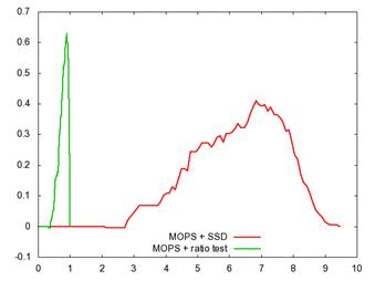
Figure 3: Threshold plot for Yosemite (left) and graf (right)

Harris Operator Results (as requested)

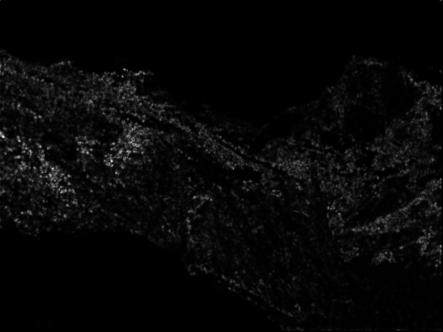
Harris Operator Results on Yosemite1.jpg

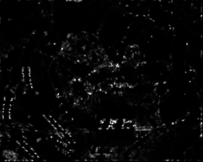
Harris Operator Results on graf image (img1.ppm)

Benchmark Results

SW = Simple Window descriptor

MY = My own descriptor

MOPS = Mops Descriptor

	Bike		Graf		Leuven		Wall
	Avg Error	Avg AUC	Avg Error	Avg AUC	Avg Error	Avg AUC	Avg Error	Avg AUC
SW + SSD	525	61.25%	270	50.43%	401	30.29%	336	47.76%
SW + ratio	525	62.15%	270	50.19%	401	48.35%	336	55.84%
MOPS + SSD	529	52.70%	294	51.77%	310	68.04%	361	63.19%
MOPS + ratio	529	57.30%	294	59.15%	310	68.09%	361	62.73%
MY + SSD	491	49.31%	264	53.01%	302	55.59%	303	54.52%
MY + ratio	491	55.04%	264	53.31%	302	60.60%	303	58.63%

Table 1: All error and AUC values averaged over images in that directory. Error is in units of pixels and AUC is area under curve.

Over all, the descriptors performed decently, but there’s still plenty of room for improvement. In almost all cases, the ratio test improved results, confirming it is the better metric to use.

The simple window’s strengths and weaknesses are most obvious. Since it only measures translational changes, it struggles on images where angles change. Hence, it performed best on bikes where the images don’t shift, but only blur. It struggled on wall and graf because of the change in the angle of the picture taken. A surprising result is how poorly it performed on the Leuven. This can partially be explained by the threshold during Harris feature selection. The threshold will discriminate greatly on the various luminous pictures, and the effect is very apparent on the results. A possible way to increase this would be to tune the threshold to see which works best for the simple window descriptor.

MOPs performed the best among the three images, and specifically performed best on the Leuven image set. This is likely because luminosity doesn’t affect MOPs as much since MOPs measures the gradient, which doesn’t change across the images. Normalizing the intensities in the MOPs descriptor likely helped in dealing directly with what the Leuven image set was testing against. MOPs also did well on the wall image set, likely highlighting that its measure radian angle helped in describing the features, since angle was the main thing being tested here. Compared to its performance on the previous two image sets, MOPs did not do that well on the bikes or graf image sets. Graf is a very difficult image set as the image warps a lot, and so there’s lots of room for mistakes. Poor performance on the bike is likely explained since blurring causes some loss of detail, and therefore, it’s harder for the MOPs descriptor to get strong gradients.

Lastly, my own descriptor did not do as well as I had hoped. Since it was modeled off of SIFT, I expected it to be robust, but it seemed to have similar trouble to the bikes and graf image sets as the MOPs descriptor did. However, it performed well on the Leuven and wall image sets for similar reasons as the MOPs.

Extra Credit

I was hoping my attempt at implementing SIFT would warrant some extra credit, but the results don’t seem to indicate the implementation was that successful. Points for effort?